At the Naval Postgraduate School we are developing a numerical model for the atmosphere called NUMA (Non-hydrostatic Unified Model of the Atmosphere). NUMA is the dynamical core inside of the Navy’s next-generation NEPTUNE weather prediction system. NEPTUNE stands for the Navy’s Environmental Prediction sysTem Using the NUMA corE. NUMA is unified across numerics (using both continuous and discontinuous Galerkin methods) and is unified across the applications (used for both regional and global modeling). In addition, NUMA has an entire suite of implicit-explicit time-integrators, iterative solvers, and preconditioners. NUMA has been shown to scale well up to the extreme limit when there is one element per processor. NUMA allows for arbitrarily high-order accuracy of the numerics and has the capacity to handle unstructured and adaptive grids.

A few weeks ago my colleague Simone Marras successfully added the capacity to simulate clouds in NUMA and ran some nice cloud simulations (see our conference paper here). This raised the question: how should we visualize our cloud simulations? I do have some experience with using the free computer graphics software Blender. For this reason I got the task to find a good way for rendering our clouds. I asked some computer graphics experts at the Naval Postgraduate School. Jeffrey Weekley from the MOVES institute recommended to use the commercial Maya® 3D computer graphics software from Autodesk®. It has been used for creating many popular movies. A full commercial license of Maya costs almost $4000. Fortunately Autodesk offers a free educational license and allows the use of this educational license for purposes directly related to research.

The difficulty with using Maya for visualizing scientific data was that I couldn’t find any instructions on how to assign our own data to the fluid objects in Maya. The movie industry would create the whole cloud directly in Maya and among scientists it seems that nobody has used Maya for this purpose. In this article I describe how to solve the difficulties that I was facing when visualizing our cloud simulation with Maya. This article is not an introduction into using Maya. There are many nice tutorials already available for getting started with Maya. If you are interested in using Maya please watch some of those basic tutorials and make yourself familiar with the GUI of Maya.

How does the data look like

Before we start using the Maya software let us first take a quick look at our data. An excellent software for taking a quick look at 3D data is Paraview®. As a first step let us take a look at our cloud at the time t=7500s from the top by plotting the isosurface of a cloud water content q_c of 0.0035 kg water per kg dry air:

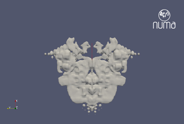
The cloud is symmetric along the x-axis because the simulation was started with a symmetric initial condition. How would a viewer at the ground see this cloud? Moving the camera to x=41.4km, y=47.7km and z=0km and targeting the camera towards the point x=0km, y=4.4km, z=8.1km with a vertical angle of view of 30.6° gives the following picture:

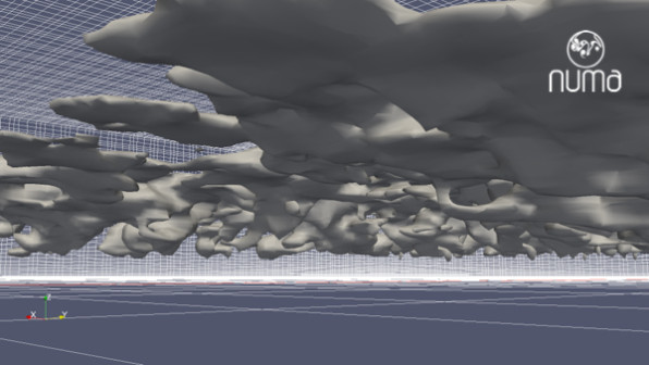
This plot includes a wireframe showing the grid on which we have our data. The grid is slightly stretched in the vertical. The horizontal size of the elements is constant. However our simulation uses four Gauss-Lobatto points inside each element for each direction. This leads to the mesh shown in the previous plot.

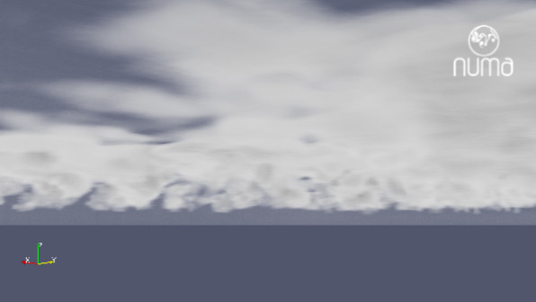
In reality clouds do not have a solid surface but are transparent at their boundaries. In Paraview this effect can be obtained by using volumetric rendering. Adjusting the opacity profile in the advanced color map settings allows to create this more cloud-like look:

The first Maya rendering

Jeffrey Weekley suggested to start by using one of the fluid examples in Maya Visor. Inside the Maya GUI you can open Visor from the menu “Window” > “General Editors” > “Visor”. In Visor select the tab “Fluid Examples” and inside this tab the folder “CloudsAndFog”. Here you can find a great set of nice ready-to-use clouds. The example which I use as a starting point is called CloudsSun.ma. Just by rendering this example with the Maya software renderer without any modifications you get the following picture:

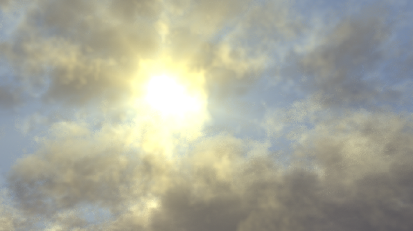
So far the cloud uses a simple vertical gradient for its density. The cloud look is then created by texturing opacity with so called “Perlin Noise”. Now we need to get the data from our scientific simulations into Maya.

Getting the data into Maya

The Visor example from the last section created a so called 3D fluid container and named it “Clouds”. This object contains a node named “CloudsShape” which can be selected in the Attribute Editor of Maya. For using our own data as the density of the fluid we need to change the “Contents Method” for Density in the Attribute Editor of the CloudsShape from “Gradient” to “Static Grid”. Now we can assign our own density to the grid by executing the following Python script in the Script Editor of Maya (menu “Window” > “General Editors” > “Script Editor”):

# Load Maya module:
import maya.cmds as cmds

# Import the data ...
# The following variables need to be created:
# npoints: total number of points in the mesh
# npx, npy, npz: number of points in x,y,z-direction
# x,y,z: arrays containing x,y,z coordinate of every point (I like the look of the cloud texture when using x,y,z in km)
# ix,iy,iz: integer arrays counting the points in x,y,z direction starting with 0
# qc: array containing the cloud water content of every point
# one possible way for ASCII files with columns separated by ',':
from pylab import *
data  = genfromtxt('cloudData.dat', skip_header=1, delimiter=',')
x = data.T[0]
y = data.T[1]
z = data.T[2]
qc = data.T[3]
ix = data.T[4]
iy = data.T[5]
iz = data.T[6]
npoints = len(x)
nx = unique(x)
ny = unique(y)
nz = unique(z)
npx = len(nx)
npy = len(ny)
npz = len(nz)

# adjust resolution and size of fluid container:
cmds.setAttr( 'CloudsShape.resolution', npy, npz, npx)
cmds.setAttr( 'CloudsShape.dimensionsW', (max(y)-min(y)))
cmds.setAttr( 'CloudsShape.dimensionsH', (max(z)-min(z)))
cmds.setAttr( 'CloudsShape.dimensionsD', (max(x)-min(x)))

# assign cloud water content as density of the fluid container:
for i in range(0, npoints-1):
    cmds.setFluidAttr( 'CloudsShape', at='density', fv=50*qc[i], xi=iy[i], yi=iz[i], zi=ix[i] )
    # Maya expects the values to be between 0 and 1. The factor 50 brings our maximum to about 0.6.

The assignment of xi=iy … in the script is not a mistake. Maya uses the y-direction for the vertical, because back in the times when computer graphics were mostly 2D it was natural to use the y direction for the vertical direction of the screen.

After executing this script Maya uses our own data for the density of the fluid container. Now we need to use our density for the opacity by changing the “Opacity Input” under “Shading” of the CloudsShape from “Y Gradient” to “Density”:

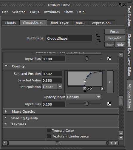
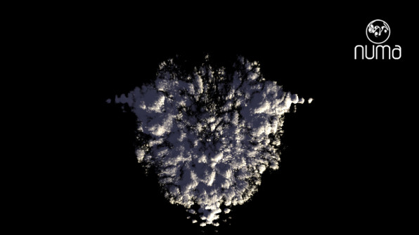
The level of cloud water content which is rendered as a cloud has to be adjusted by changing the “Input Bias”. The look of our cloud can be adjusted by changing the opacity profile (the curve shown in the screenshot of the Attribute Editor). We can speed up the rendering significantly by deactivating all the options under “Render Stats” of our CloudsShape in the Attribute Editor except for the “Primary Visibility”. Also it is useful to start with a low resolution version of our data until we have everything set up nicely. For the final picture we need to remember to switch back to using our full data. By replacing the sun with directional light coming from the bottom right I get the following rendering when using the top camera:

Having the directional light coming from the top and adding again a sun next to the cloud produces the following rendering:

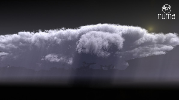
The vertical lines below the cloud look almost like rain but are actually shadows created by the directional light. The amount of dust surrounding the cloud can be modified by adjusting the bottom left value in the opacity profile (see screenshot of Attribute Editor above).

Visualizing rain

For visualizing the rainfall out of the cloud we need to find a way of rendering precipitation streaks (so called virga). I couldn’t find any example of how to render virga in Maya. Our simulation gives us for each of our grid points not only the cloud water content but also the rain water content. We can use a 3D fluid container like the one for the cloud. In the same way as with the cloud we can load our rain water content as density into this new fluid container for the rain. For getting a rain-like look we need to adjust the colors under “Color” and “Incandescence” in the Attribute Editor of our newly created “RainShape”. For giving the rain the look of vertical streaks I used “Volume Wave” for the texture type with a texture scale in vertical (y) direction of 1000. This makes the texture a purely horizontal wave. The look of the rain texture can be adjusted by changing the amplitude and frequency of the texture.

So far the renderings look more like night scenes. For making it look even more like a night scene I changed the color of the halo and glow of the sun (Attribute Editor under the opticalFX-tab) to some bluish colors. Adding a lens flare and a dark blue background in the Adobe® Photoshop® software and adding a small amount of vignetting in the Lightroom® software leads to the following result:

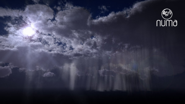
The amount of rain visible in our rendering can be changed by adjusting the input bias of the opacity of our “RainShape”.

Building an environment

Rendering night scenes of our cloud has the advantage that we don’t need any landscape in front of the cloud for making it look real. How can we render a realistic looking day scene? The easiest option seems to be: take a real photo with a blue sky, extract the landscape from the picture (e.g. with Gimp or Photoshop), put the landscape in front of the cloud and the sky behind the cloud. Here is a photo that I took last Monday (March 10th, 2014) in Pacific Grove:

In Maya photos can be added by creating “Image Planes” in the Attribute Editor of the “CameraShape” node of our camera. I created one image plane in front of my cloud and one behind it. My setting can be seen in the following screenshot of Maya:

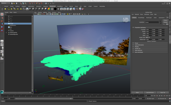
My camera is in the screenshot at the bottom left. I placed the sun between the first image plane and the camera for having some sun rays and lens flares covering the entire rendering. Rendering this scene leads to the following result:

Compared to the Paraview volume rendering the results with Maya look quite different because Maya computes shadows which the cloud casts onto itself. Therefore some details of the cloud are not visible in Maya because they are hidden in a shadow of the cloud. Here is a direct comparison:

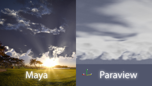
The cloud looks vertically stretched in Maya. This is not a mistake of Maya. For keeping our scripts simple I ignored the vertical stretching of our grid and used our data as if it was given on a uniform mesh. Of course we could easily correct this and evaluate the polynomials of our Spectral Element method at any point we want.

Except for the vertical stretching the shape of the cloud is very similar in Maya and Paraview. We expect the remaining slight difference to come from slightly different opacity profiles in the two softwares. Another main difference between Paraview and Maya is the speed at which the rendering is done: the Maya software renderer needs almost 1 hour on my laptop for our full resolution data whereas Paraview does its volume rendering within less than a minute. For me Paraview is the perfect choice for a quick look at the data whereas Maya is the perfect choice for making the cloud look as realistic as possible.

Autodesk screen shots reprinted with the permission of Autodesk, Inc.
Autodesk and Maya are registered trademarks or trademarks of Autodesk, Inc., and/or its subsidiaries and/or affiliates in the USA and other countries.
Adobe, Photoshop and Lightroom are either registered trademarks or trademarks of Adobe Systems Incorporated in the United States and/or other countries.